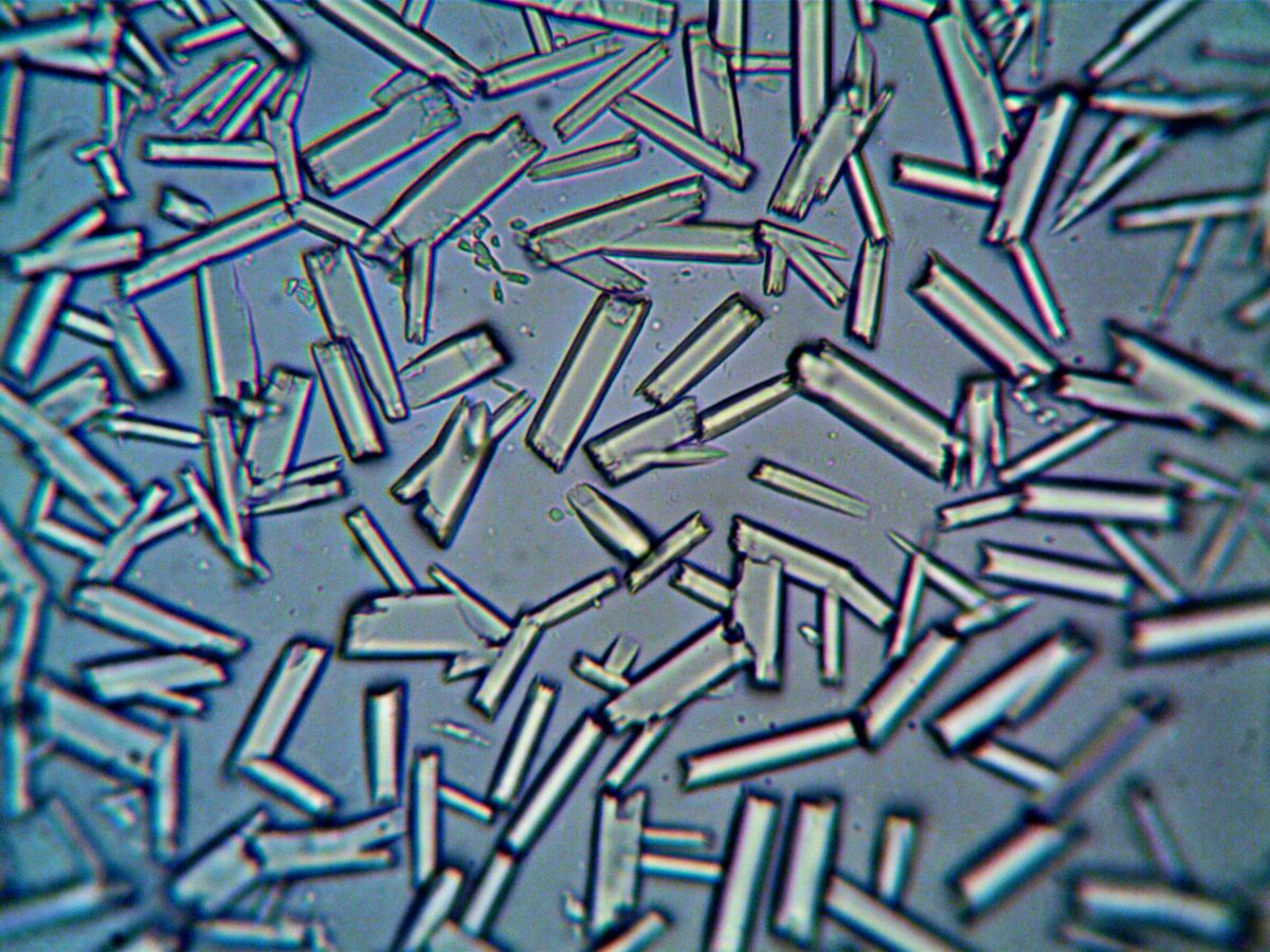
Laser diffraction measures particle sizes by reading how a laser beam scatters off particles in suspension. Shine a laser through a cloud of particles, and the light spreads into a pattern of rings and patches. Large particles scatter the light at tight angles close to the beam direction. Small particles throw the light out at wider angles. By capturing the complete angular pattern and matching it to known optical models, a laser diffraction particle size analyser can report how many particles there are at every size — from 10 nanometres to several millimetres — in under a minute.
Think of it like throwing stones of different sizes into a pond. A large stone produces a tight cluster of big ripples. A handful of gravel produces many small ripples that spread in all directions. If you stood above the pond and measured the pattern of ripples, you could work out the mix of stone sizes. Laser diffraction does the same thing, but with light scattering off particles instead of stones hitting water.
How a laser diffraction particle size analyzer works
Every laser diffraction instrument has three main parts: a light source, a sample handling system, and a detector.
| Component | Function |
|---|---|
| Light source | One or more lasers (red He-Ne at 633 nm, blue diode at 470 nm or shorter) to cover a wide size range |
| Sample dispersion unit | Circulates the sample as a liquid suspension, dry powder flow, or aerosol stream through the laser beam |
| Detector array | A set of photosensitive elements arranged in rings and wedges that measure scattered light intensity at multiple angles simultaneously |
The laser beam is expanded and collimated so it illuminates the entire sample volume uniformly. Particles in the beam scatter the light in all directions. The undiffracted beam passes through a central hole in the detector array and is captured by a beam stop. The detector elements record the intensity at angles from about 0.02° to over 140°.
The raw data is a plot of scattered light intensity against angle — a smooth curve that encodes the entire particle size distribution. The next step is to decode it using an optical model.
Fraunhofer versus Mie: which theory to use
There are two mathematical models for converting the scattering pattern into particle sizes: Fraunhofer diffraction theory and Mie theory.
Fraunhofer approximation treats every particle as an opaque disc and only considers light diffracted at the particle edge. It ignores what happens to light that passes through the particle — refraction, reflection, and absorption. Its main advantage is simplicity: it requires no knowledge of the material's optical properties. But it is only accurate when particles are at least 10 times larger than the laser wavelength (about 10 µm for a red laser). For smaller or transparent particles, Fraunhofer underestimates the fine fraction.
Mie theory is the full solution to Maxwell's equations for light scattering by spherical particles. It accounts for diffraction at the particle edge, refraction through the particle, reflection from the surface, and absorption inside the material. Mie theory is accurate from nanometres to millimetres, but it requires three pieces of information: the real refractive index of the particle, the imaginary refractive index (absorption coefficient), and the refractive index of the dispersant.
The rule of thumb: use Fraunhofer when particles are large (>50 µm) and opaque. Use Mie for everything else — especially particles below 50 µm, transparent particles, and coloured materials. Modern analysers automatically switch between the two based on the user's input.
Sample preparation: wet versus dry dispersion
Getting the measurement right starts with getting the particles into the laser beam in a well-dispersed state. Agglomerated particles read as single large particles, which ruins the result. There are two main approaches:
Wet dispersion suspends the powder in a liquid (usually water, sometimes isopropanol or oil). An ultrasonic probe breaks up agglomerates, and a stirrer keeps the particles circulating through the measurement cell. Wet dispersion is ideal for samples that are already in suspension, for materials that are sensitive to mechanical stress, and for high-precision pharmaceutical analysis.
Dry dispersion uses compressed air or a Venturi system to draw powder from a hopper and accelerate it through the laser beam. Particles collide with each other and with the walls of the dispersion nozzle, breaking up agglomerates. Dry dispersion is faster (no liquid preparation), avoids solubility issues, and is the method of choice for production-line quality control.
The ISO standard 13320:2020 specifies the requirements for both methods — including acceptable obscuration levels, measurement repeatability, and instrument validation procedures.
What the results mean: D10, D50, D90
Laser diffraction reports particle size as a volume-weighted distribution. The most widely used metrics are:
- D10 — 10% of the total sample volume consists of particles smaller than this diameter
- D50 — the median diameter; half the volume is above, half below
- D90 — 90% of the volume is below this diameter
- Span — (D90 − D10) / D50 — a measure of the width of the distribution
A worked example: suppose a pharmaceutical powder has D10 = 2.1 µm, D50 = 5.8 µm, and D90 = 12.4 µm. The span is (12.4 − 2.1) / 5.8 = 1.78. A span close to 1 means a narrow distribution; a larger span means a broader mix of particle sizes.
The distribution can also be plotted as a density curve (showing the relative volume at each size) or a cumulative curve (showing the percentage below each size). Both are standard outputs from modern analysers.
5 applications of laser diffraction
1. Pharmaceutical manufacturing. Active pharmaceutical ingredients must have tightly controlled particle sizes to ensure consistent dissolution rates and bioavailability. Laser diffraction is used in R&D and quality control for API powders, excipients, and inhalation aerosols.
2. Cement and construction. The particle size distribution of cement powder directly affects the setting time and strength of concrete. Laser diffraction is the standard quality control method in cement plants worldwide.
3. Mining and minerals. From iron ore to clays, laser diffraction measures the grind size and monitors mill performance. The technique replaced the traditional sieve-and-sedimentation method in most modern labs.
4. Food and beverages. Chocolate, coffee, milk powder, and flour all have particle sizes that affect taste, texture, and processing behaviour. Laser diffraction provides rapid quality checks on production lines.
5. Environmental monitoring. Soil texture analysis, sediment transport studies, and aerosol characterisation all rely on laser diffraction for fast, reproducible particle sizing across a wide dynamic range.
Common misconception: laser diffraction measures particle shape
Laser diffraction does not measure particle shape. The Mie and Fraunhofer models assume spherical particles, and the result is always an equivalent spherical diameter — the diameter of a sphere that would produce the same scattering pattern. Non-spherical particles produce broader, more diffuse scattering patterns, and the reported size distribution will differ from what microscopy would show. For this reason, laser diffraction results should always be interpreted alongside shape information from imaging when particle morphology matters.
For more on the fundamental physics of diffraction, see what is diffraction and examples of diffraction. The guide on Fraunhofer vs Fresnel diffraction explains the difference between the far-field model used in laser diffraction and near-field diffraction.
External resources
- Wikipedia: Laser diffraction analysis — comprehensive overview of the method and theory
- Anton Paar Wiki: Laser diffraction for particle sizing — practical guide with diagrams of instrument components
- ISO 13320:2020 — Particle size analysis by laser diffraction — international standard for the technique
Frequently Asked Questions
What is laser diffraction analysis?
Laser diffraction analysis is a technique that measures particle size distributions by directing a laser beam through a dispersed sample and analysing the angular pattern of scattered light. Large particles scatter light at small angles relative to the beam, while small particles scatter at large angles. The measured intensity pattern is compared against optical models (Mie theory or Fraunhofer approximation) to calculate the size distribution.
What is the difference between Fraunhofer and Mie theory in laser diffraction?
Fraunhofer diffraction theory assumes particles are opaque discs and only considers light diffracted at the particle edge. It does not require knowledge of the particle's optical properties but is only accurate for particles at least 10 times larger than the laser wavelength. Mie theory accounts for diffraction, refraction, reflection, and absorption within and at the surface of particles. It is accurate across the full size range but requires the complex refractive index of the material.
What particle sizes can laser diffraction measure?
Modern laser diffraction instruments can measure particles from about 10 nanometres up to several millimetres — a dynamic range of about five orders of magnitude. The upper limit depends on the optical configuration: instruments using wide-angle detector arrays and multiple light sources (red and blue lasers) achieve the widest range. The lower limit is set by the signal-to-noise ratio of small-particle scattering.
How does a laser diffraction particle size analyzer work?
A laser diffraction analyzer consists of three main parts: a laser source (typically He-Ne or laser diode), a sample dispersion unit, and a multi-element detector array. The laser beam passes through the dispersed sample. Particles scatter the light, and the detector array measures the angular intensity pattern. A computer applies Mie theory or the Fraunhofer approximation to transform the scattering pattern into a volume-weighted particle size distribution.
What is D50 in laser diffraction results?
D50 is the median particle diameter: 50% of the sample volume consists of particles smaller than this value, and 50% are larger. It is the most commonly reported metric from laser diffraction analysis. Other common metrics include D10 (10% below this size) and D90 (90% below this size). The span of the distribution is calculated as (D90 − D10) / D50.
What are the advantages of laser diffraction over sieving?
Laser diffraction is faster (results in under a minute vs hours for sieving), covers a wider size range (10 nm to several mm vs ~20 µm to 125 mm for sieving), requires less sample material, provides continuous distribution data rather than discrete size fractions, and can measure wet or dry samples. It is also more repeatable because it samples thousands of particles per measurement.

About Umar Farooq
Umar Farooq writes in-depth guides on the physics of light and optics — from reflection, refraction, and lenses to diffraction, lasers, and fiber optics, explained from first principles.
Read more about Umar Farooq →